Graphs 1: Introduction with BFS & DFS
Graphs Introduction
Introduction
Graph: It is a collection of nodes and edges.
Some real life examples of Graph -
- Network of computers
- A Website
- Google Maps
- Social Media


Types of Graph
Cyclic Graph
A cyclic graph contains at least one cycle, which is a closed path that returns to the same vertex.
Diagram:
A -- B
|    |
|    |
D -- C
Acyclic Graph
An acyclic graph has no cycles, meaning there are no closed paths in the graph.
Diagram:
A -- B
|    |
D    C
Directed Graph (Digraph)
In a directed graph, edges have a direction, indicating one-way relationships between vertices.
Diagram:
A --> B
|     |
v     v
D --> C
Undirected Graph
In an undirected graph, edges have no direction, representing symmetric relationships between vertices.
Diagram:
A -- B
|    |
|    |
D -- C
Connected Graph
A connected graph has a path between every pair of vertices, ensuring no isolated vertices.
Diagram
A -- B
|
D -- C
Disconnected Graph
A disconnected graph has at least two disconnected components, meaning there is no path between them.
Diagram:
A -- B    C -- D
|              |
E -- F    G -- H
Weighted Graph
In a weighted graph, edges have associated weights or costs, often used to represent distances, costs, or other metrics.
Diagram (Undirected with Weights):
A -2- B
|     |
1     3
|     |
D -4- C
Unweighted Graph
An unweighted graph has no associated weights on its edges.
Diagram (Undirected Unweighted):
A -- B
|
D -- C
Degree of a Vertex
The degree of a vertex is the number of edges incident to it.
Diagram:
   B
   |
A--C--D
Outdegree of a Vertex
The outdegree of a vertex in a directed graph is the number of edges leaving that vertex.
Diagram:
A --> B
|     |
v     v
D --> C
Simple Graph
A simple graph has no self-loops or multiple edges between the same pair of vertices.
Diagram:
A -- B
|
D -- C
How to store a graph
Graph:
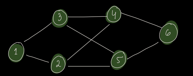
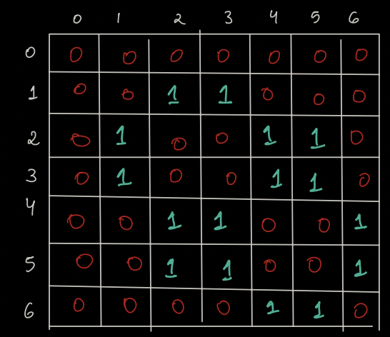
Adjacency Matrix:
All the edges in above graph has equal weights.
In adjacency matrix, mat[i][j] = 1, if there is an edge between them else it will be 0.
Pseudocode:
int N, M
int mat[N+1][M+1] = {0}

for(int i=0; i < A.size(); i++) {
    u = A[i][0];
    v = A[i][1];

    mat[u][v] = 1
    mat[v][u] = 1
}
Note: In case of weighted graph, we store weights in the matrix.
Advantage: Easy to update new edges.
Disadvantage: Space wastage because of also leaving space for non-exitent edges. Moreover, If N<=105, it won't be possible to create matrix of size 10^10. It is possible only if N <= 103
Space Complexity: O(N2)
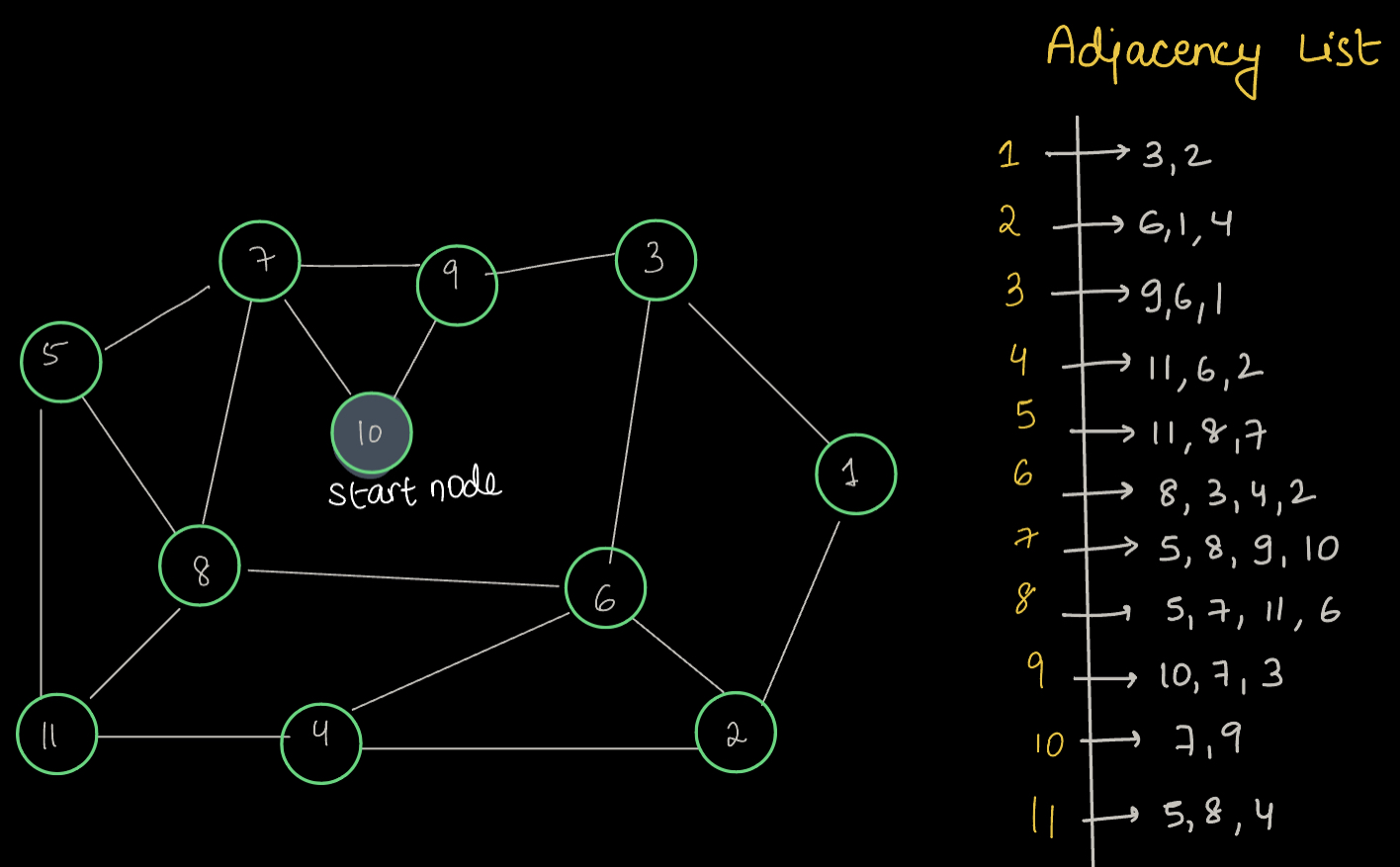
2. Adjacency List:
An adjacency list is a common way to represent a graph in computer science. It's used to describe which nodes (or vertices) in the graph are connected to each other. Here's how it works:
Graph:
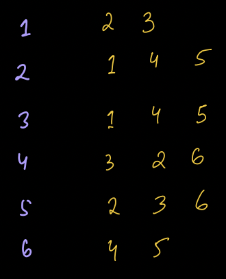
Adjacency List:
Stores the list of nodes connected corresponding to every node.
We can create map of
map<int, list<int>> graph;

OR

list<int> graph[]
Pseudocode:
int N
int M
list < int > graph[N + 1]
for (int i = 0; i < A.size(); i++) {
    u = A[i][0]
    v = A[i][1]

    graph[u].add(v)
    graph[v].add(u)
}
- We refer the adjacent nodes as neighbours.
Question
Consider a graph contains V vertices and E edges. What is the Space Complexity of adjacency list?
Choices
- O(V2)
- O(E2)
- O(V + E)
- O(V*E)
Space is defined by the edges we store. An Edge e comprise of two nodes, a & b. For a, we store b and for b, we store a. Hence, 2 * E.
Now, we are doing this for every node, hence +V.
Space Complexity: O(V+E)
Graph traversal algorithm - DFS
There are two traversal algorithms - DFS (Depth First Search) and BFS(Breadth First Search).
In this session, we shall learn DFS and in next, BFS.
DFS
Depth-First Search (DFS) is a graph traversal algorithm used to explore all the vertices and edges of a graph systematically. It dives deep into a graph as far as possible before backtracking, hence the name "Depth-First." Here's a basic explanation of the DFS process with an example:
Process of DFS:
- Start at a Vertex: Choose a starting vertex (Any).
- Visit and Mark: Visit the starting vertex and mark it as visited.
- Explore Unvisited Neighbors: From the current vertex, choose an unvisited adjacent vertex, visit, and mark it.
- Recursion: Repeat step 3 recursively for each adjacent vertex.
- Backtrack: If no unvisited adjacent vertices are found, backtrack to the previous vertex and repeat.
- Complete When All Visited: The process ends when all vertices reachable from the starting vertex have been visited.
Example/Dry-run:
Consider a graph with vertices A, B, C, D, E connected as follows:
A ------ B
|        |
|        |
|        |
C        D
\
 \
  \
   \
    E
DFS Traversal:
- Start at A: Visit A.
- Visit Unvisited Neighbors of A:
- Go to B (unvisited neighbor of A).
- Visit B.
- Visit Unvisited Neighbors of B:
- Go to D (unvisited neighbor of B).
- Visit D.
- Backtrack to B: Since no more unvisited neighbors of D.
- Backtrack to A: Since no more unvisited neighbors of B.
- Visit Unvisited Neighbors of A:
- Go to C (unvisited neighbor of A).
- Visit C.
- Visit Unvisited Neighbors of C:
- Go to E (unvisited neighbor of C).
- Visit E.
- End of DFS: All vertices reachable from A have been visited.
DFS Order: The order of traversal would be: A → B → D → C → E.
Pseudocode:
We'll take a visited array to mark the visited nodes.
// Depth-First Search function
int maxN = 10 ^ 5 + 1
list < int > graph[maxN];
bool visited[maxN];

void dfs(int currentNode) {
    // Mark the current node as visited
    visited[currentNode] = true;

    // Iterate through the neighbors of the current node
    for (int i = 0; i < graph[currentNode].size(); i++) {
        int neighbor = graph[u][i];
        // If the neighbor is not visited, recursively visit it

        if (!visited[neighbor]) {
            dfs(neighbor);
        }
    }
}
Question
Time Complexity for DFS?
Choices
- O(V + E)
- O(V)
- O(2E)
Explanation:
The time complexity of the DFS algorithm is O(V + E), where V is the number of vertices (nodes) in the graph, and E is the number of edges. This is because, in the worst case, the algorithm visits each vertex once and each edge once.
Space Complexity: O(V)
Problem 1 Detecting Cycles in a Directed Graph
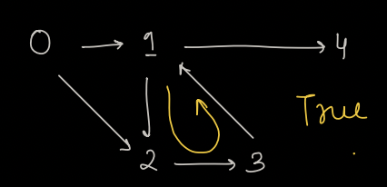
Check if given graph has a cycle?
Examples
1) 
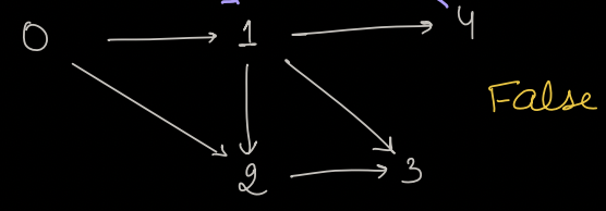
2) 
Warning
Please take some time to think about the solution approach on your own before reading further.....
Approach
Apply DFS, if a node in current path is encountered again, it means cycle is present! With this, we will have to keep track of the path.
Example 1:
Say we start at 0 -> 1 -> 3
path[] = {0, 1, 3}
Now, while coming back from 3, we can remove the 3 from path array.
path[] = {0, 1}
Now, 0 -> 1 -> 2 -> 3
path[] = {0, 1, 2, 3} [Here, we came back to 3, but via different path, which is not an issue for us]
Example 2:
Say we start at 0 -> 1 -> 2 -> 3
path[] = {0, 1, 2, 3}
Now, from 3, we come back to 1.
path[] = {0, 1, 2, 3, 1} [But 1 is already a part of that path, which means cycle is present]
Pseudocode
list < int > graph[] //filled
bool visited[] = {0}
int path[N] = {0}

bool dfs(int u) {
    visited[u] = true
    path[u] = 1

    for (int i = 0; i < graph[u].size(); i++) {
        int v = graph[u][i]
        if (path[v] == 1) return true
        else if (!visited[v] && dfs(v)) {
            return true
        }
    }
    path[u] = 0;
    return false;
}
Complexity
Time Complexity: O(V + E)
Space Complexity: O(V)
Problem 2 Number of Islands Statement and Approach
You are given a 2D grid of '1's (land) and '0's (water). Your task is to determine the number of islands in the grid. An island is formed by connecting adjacent (horizontally or vertically) land cells. Diagonal connections are not considered.
Given here if the cell values has 1 then there is land and 0 if it is water, and you may assume all four edges of the grid are all surrounded by water.
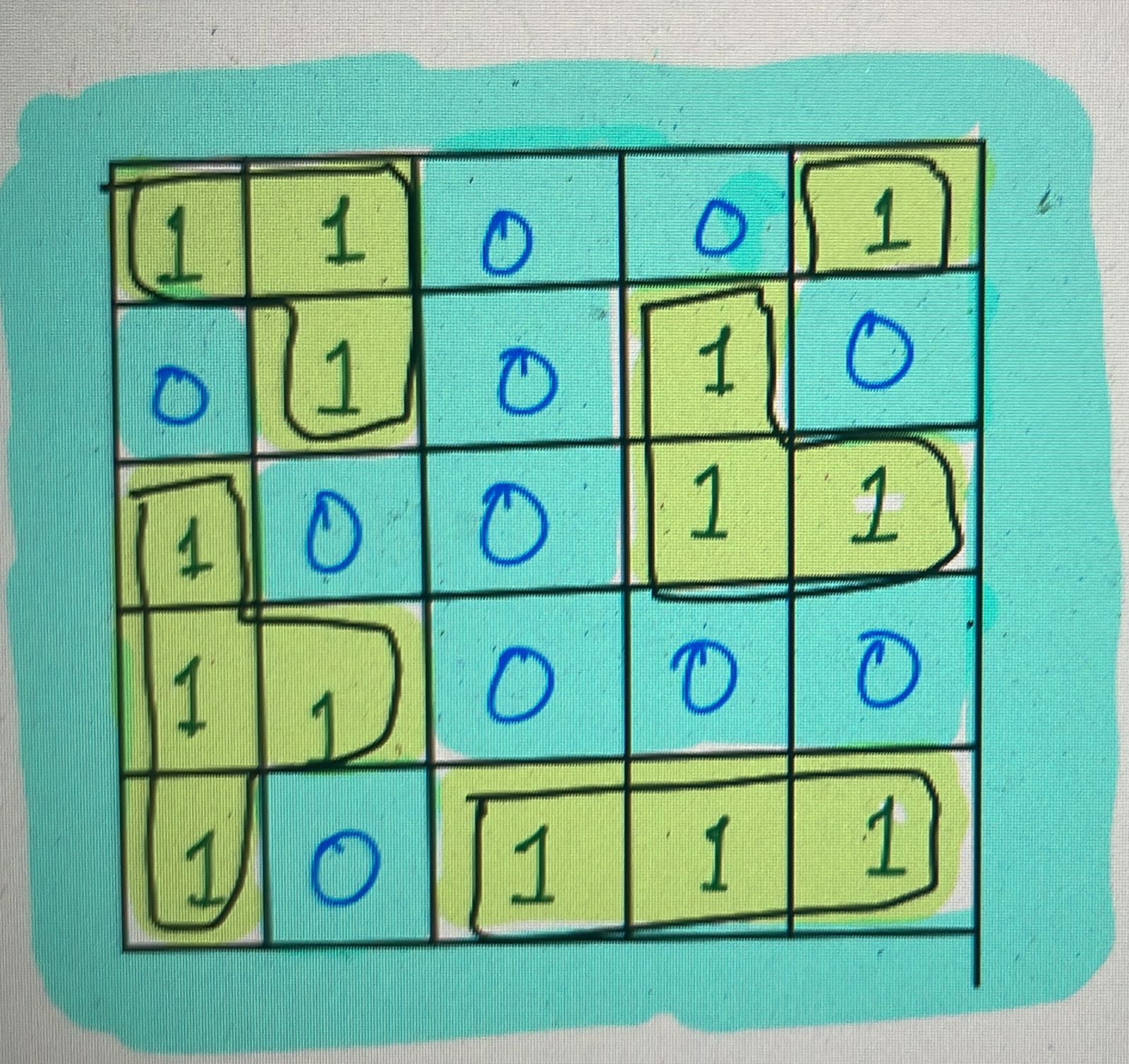
In this case we can see that our answer is 5.
Que: Do we need adjacency list ?
Ans: No, since the information is already present in form of matrix which can be utilised as it is.
Warning
Please take some time to think about the solution approach on your own before reading further.....
Approach:
Set a Counter: Start with a counter at zero for tracking island count.
Scan the Grid: Go through each cell in the grid.
Search for Islands: When you find a land cell ('1'), use either BFS or DFS to explore all connected land cells.
Mark Visited Cells: Change each visited '1' to '0' during the search to avoid recounting.
Count Each Island: Increase the counter by 1 for every complete search that identifies a new island.
Finish the Search: Continue until all grid cells are checked.
Result: The counter will indicate the total number of islands.
Number of Islands Dry Run and Pseudocode
Dry-Run:
[
 ['1', '1', '0', '0', '0'],
 ['1', '1', '0', '0', '0'],
 ['0', '0', '0', '0', '0'],
 ['0', '0', '0', '1', '1']
]
- Initialize variable islands = 0.
- Start iterating through the grid:
- At grid[0][0], we find '1'. Increment islands to 1 and call visitIsland(grid, 0, 0).
- visitIsland will mark all connected land cells as '0', and we explore the neighboring cells recursively. After this, the grid becomes:
[
 ['0', '0', '0', '0', '0'],
 ['0', '0', '0', '0', '0'],
 ['0', '0', '1', '0', '0'],
 ['0', '0', '0', '1', '1']
]
- Continue iterating through the grid:
- At grid[2][2], we find '1'. Increment islands to 2 and call visitIsland(grid, 2, 2).
- visitIsland will mark connected land cells as '0', and we explore the neighboring cells recursively. After this, the grid becomes:
[
 ['0', '0', '0', '0', '0'],
 ['0', '0', '0', '0', '0'],
 ['0', '0', '0', '0', '0'],
 ['0', '0', '0', '1', '1']
]
- Continue the iteration.
- At grid[3][3], we find '1'. Increment islands to 3 and call visitIsland(grid, 3, 3).
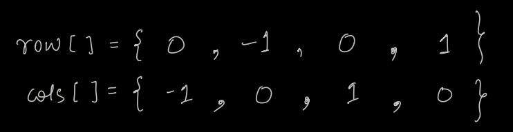
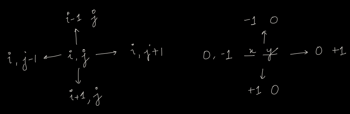
We can visit only 4 coordinates, considering them to be i, j; it means we can visit (i,j-1), (i-1, j), (i, j+1), (i+1, j)
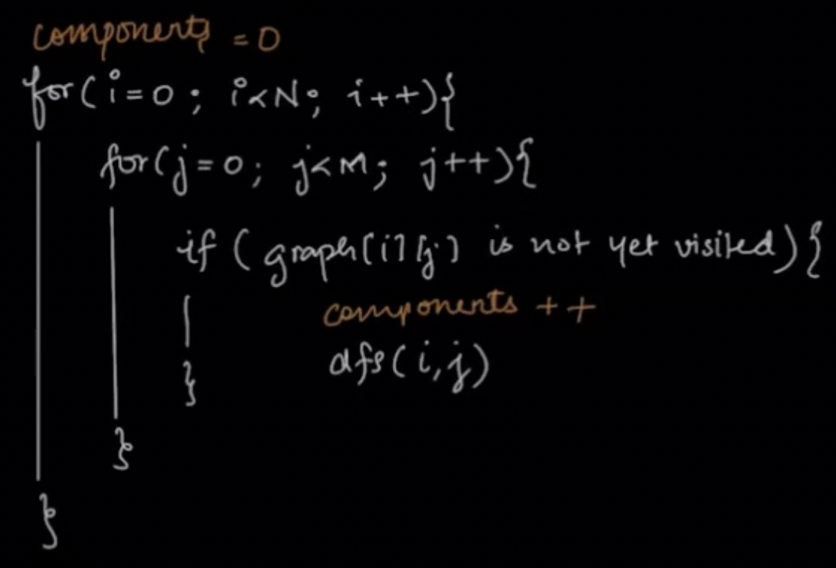
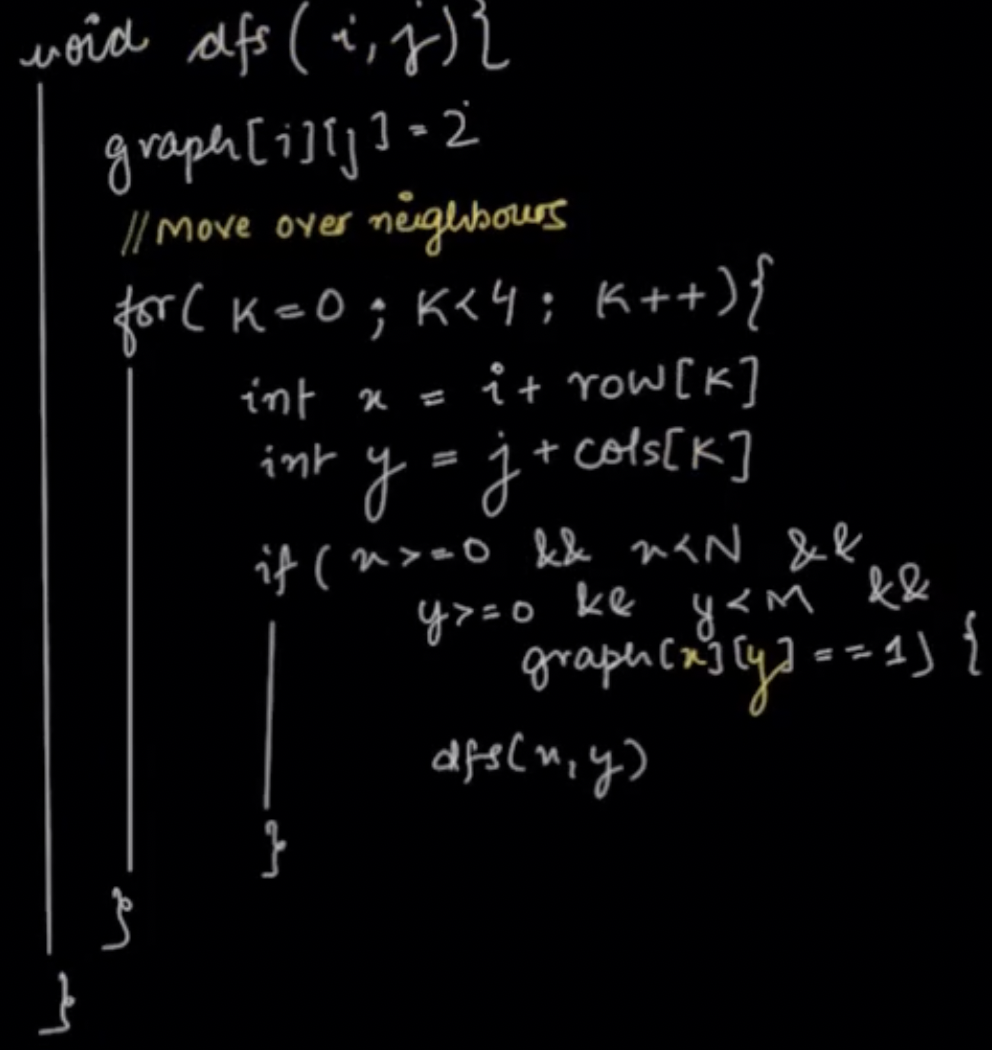
Pseudocode