Searching 2: Binary Search Problems¶

Understanding Binary Search¶

Introduction:¶

We will continue with our second lecture on Binary Search. In our previous session, we explored the fundamental concepts of this efficient searching algorithm. Today, we will dive even deeper into the world of binary search, uncovering advanced techniques and applications that expand its capabilities.

In this lecture, we will build upon the foundation laid in the first session. We'll delve into topics such as binary search on rotated arrays, finding square root using binary search etc and addressing various edge cases and challenges that may arise during binary search implementation.

Pseudocode¶

function binarySearch(array, target):
    left = 0
    right = length(array) - 1

    while left <= right:
        mid = left + (right - left) / 2

        if array[mid] == target:
            return mid
        else if array[mid] < target:
            left = mid + 1
        else:
            right = mid - 1

    return NOT_FOUND

Use Cases:¶

Binary search has numerous applications, including:

Searching in databases.
Finding an element in a sorted array.
Finding an insertion point for a new element in a sorted array.
Implementing features like autocomplete in search engines.

Question¶

In what scenario does Binary Search become ineffective?

Choices

When the dataset is unsorted.
When the dataset is extremely large.
When the dataset is sorted in descending order.
When the dataset contains only unique elements.

Problem 1 Searching in Rotated Sorted Arrays¶

Introduction:¶

We'll explore the fascinating problem of searching in rotated sorted arrays using the Binary Search algorithm. This scenario arises when a previously sorted array has been rotated at an unknown pivot point. We'll discuss how to adapt the Binary Search technique to efficiently find a target element in such arrays.

Scenario:¶

Imagine you have an array that was sorted initially, but someone rotated it at an unknown index. The resulting array is a rotated sorted array. The challenge is to find a specific element in this rotated array without reverting to linear search.

Example: Finding an Element in a Rotated Array¶

Suppose we have the following rotated sorted array:

Original Sorted Rotated Array: [4, 5, 6, 7, 8, 9, 1, 2, 3]

Let's say we want to find the element 7 within this rotated array using a brute-force approach (Linear Search).

Brute-Force Approach:¶

Initialize a variable target with the value we want to find (e.g., 7).
Loop through each element in the array one by one, starting from the first element.
Compare the current element with the target:
If the current element matches the target, we have found our element, and we can return its index.
If the current element does not match the target, continue to the next element.
Repeat step 3 until we either find the target or reach the end of the array without finding it.

Adapting Binary Search:¶

While the array is rotated, we can still leverage the divide-and-conquer nature of Binary Search. However, we need to make a few adjustments to handle the rotation.

Intution:

In a rotated sorted array, elements were initially sorted in ascending order but have been rotated at some point.
Let's asusme array contain distinct elements only.
The goal is to find a specific target element within this rotated array.
The key to binary search in a rotated array is to determine the pivot point, which is where the array rotation occurred.
The pivot point is essentially the maximum element in the array.
Once you've identified the pivot point, you have split the array into two subarrays, each of which is sorted.
Then you can apply individual binary search in both the parts, and find the target element.
Another Idea of Doing it in one Binary Search we'll discuss below
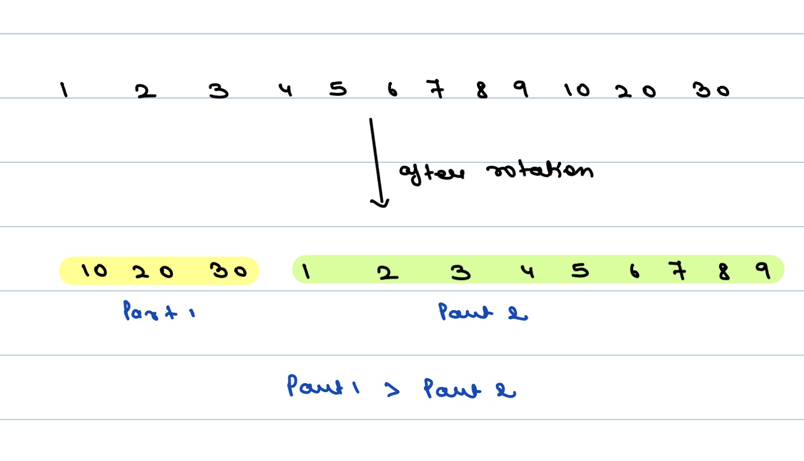
Partitioning of Rotated Sorted Array:
A rotated sorted array can be visualized as being split into two parts: part 1 and part 2.
Crucially, both part 1 and part 2 are sorted individually, but every element in part 1 is greater than those in part 2 due to the rotation.
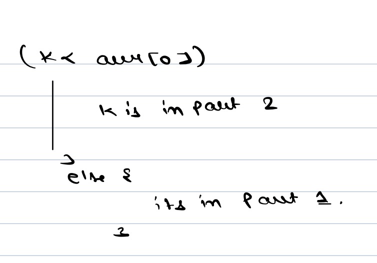
Identifying Target's Part
To determine which part the Target belongs to (part 1 or 2), compare it with the 0^th element.
If the midpoint is greater than (also equals to) the 0^th element, then it belongs to part 1. Otherwise, it's in part 2.

Identifying Midpoint's Part:
To determine which part the midpoint belongs to (part 1 or 2), compare it with the 0^th element.
If the midpoint is greater than (also equals to) the 0^th element, then it belongs to part 1. Otherwise, it's in part 2.
Midpoint vs Target:
- If the midpoint is the equals to the target, you've found it.
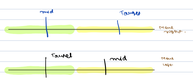
- If not, then check if the target lies in the same part as the midpoint. If yes, both target and midpoint is within the same sorted part, perform a binary search in that part to move your midpoint towards the target.

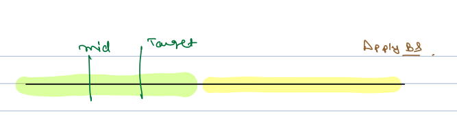
* If no, move your search towards the other part, effectively approaching the midpoint towards target.

Iterative Process:
- Continue adjusting your boundaries based on the decisions made in the previous step until you either find the target or exhaust your search space.
- Result:
- Return the index of the target if found, or -1 if not.

Algorithm:

Initialize left to 0 and right to len(nums) - 1.
While left is less than or equal to right, do the following:
Calculate the middle index mid as left + (right - left)/2.
If nums[mid] is equal to the target, return mid as the index of the target.
Check if the target is less than nums[0] (indicating it's on part 2):
If target < nums[0], check if nums[mid] is greater than or equal to nums[0]:
If true, update left to mid + 1 to search the right half.
If false, update right to mid - 1 based on target's relation to nums[mid].
If the target is greater than or equal to nums[0] (indicating it's on the left side of the pivot):
If target >= nums[0], check if nums[mid] is less than nums[0]:
If true, update right to mid - 1 to search the left half.
If false, update left to mid + 1 based on target's relation to nums[mid].
Repeat steps 2-6 until left is less than or equal to right.
If the loop exits without finding the target, return -1 to indicate the target is not in the array.

Example:¶

Scenario:

Consider the rotated sorted array [4, 5, 6, 7, 0, 1, 2] and our target is 0.

Solution:

Using the provided algorithm:
Initialize left to 0 and right to 6.
Calculate mid as (left + right) // 2, which is 3.
Check if nums[mid] (element at index 3) is equal to the target (0). It's not equal.
Check if target (0) is less than nums[0] (4). It's not.
Check if nums[mid] (7) is greater than or equal to nums[0] (4). It's true.
Update left to mid + 1, making left equal to 4.
Calculate mid as (left + right) // 2, which is 5.
Check if nums[mid] (element at index 5) is equal to the target (0). It is equal.
Return mid, which is 5.

We found the target 0 at index 5.

Searching in Rotated Sorted Arrays Pseudocode¶

Pseudocode:¶

function searchRotatedArray(nums, target):
    left = 0
    right = length(nums) - 1

    while left <= right:
        mid = left + (right - left) / 2

        if nums[mid] == target:
            return mid

        if target < nums[0]:
            if nums[mid] >= nums[0]:
                left = mid + 1
            else:
                if nums[mid] < target:
                    left = mid + 1
                else:
                    right = mid - 1
        else:
            if nums[mid] < nums[0]:
                right = mid - 1
            else:
                if nums[mid] < target:
                    left = mid + 1
                else:
                    right = mid - 1

    return -1

Complexity Analysis:¶

The time complexity of this modified Binary Search algorithm is still O(log n), making it efficient even in rotated sorted arrays.

Reason:

Divide and Conquer:
The algorithm works by repeatedly dividing the search space in half. In each step, it either eliminates half of the remaining elements or finds the target element. This is a characteristic of binary search, which has a time complexity of O(log N).
Comparison Operations:
The main operations within each iteration are comparisons of the target element with the middle element. Since we're dividing the array in half with each comparison, we need at most O(log N) comparisons to find the element or determine that it's not present.
No Need to Examine All Elements:
Unlike linear search, which would require examining all N elements in the worst case, binary search significantly reduces the number of elements that need to be considered, leading to a logarithmic time complexity.

Question¶

In the problem of searching for a target element in a rotated sorted array, what advantage does Binary Search offer over Linear Search?

Choices

Binary Search doesn't require any comparisons.
Binary Search works faster on unsorted arrays.
Binary Search divides the search space in half with each step.
Binary Search is always faster than Linear Search.

Explanation:

Binary Search offers a significant advantage over Linear Search when searching in a rotated sorted array. With each step, Binary Search efficiently narrows down the search interval by dividing it in half, greatly reducing the number of elements under consideration. This characteristic leads to a time complexity of O(log n), making Binary Search much faster compared to Linear Search's O(n) time complexity, especially for larger arrays.

Problem 2 Finding the square root of a number¶

Introduction:¶

Now, we'll explore a fascinating application of Binary Search: finding the square root of a number. The square root operation is a fundamental mathematical operation, and we'll see how Binary Search helps us approximate this value with great efficiency.

Motivation:¶

Imagine you're working on a mathematical problem or a scientific simulation that requires the square root of a number. Calculating square roots manually can be time-consuming, and a reliable and fast method is needed. Binary Search provides an elegant way to approximate square roots efficiently.

Brute-Force Algorithm to Find the Square Root:¶

Input Validation: If it's negative, return "Undefined" because the square root of a negative number is undefined.
Special Cases: If x is 0 or 1, return x because the square root of 0 or 1 is the number itself.
Initialize Guess: Start with an initial guess of 1.
Check if the square of the current guess is less than or equal to x. If it is, continue to the next step. If not, exit the loop.
Increment Guess: Increment the guess by 1.
Exit Loop: When the loop exits, it means guess * guess exceeds x. The square root is approximated as guess - 1 because guess at this point is the smallest integer greater than or equal to the square root of x.
Return Result: Return guess - 1 as the square root of x.

function sqrt_with_floor(x):
    if x < 0:
        return "Undefined"  // Square root of a negative number is undefined

    if x == 0 or x == 1:
        return x  // Square root of 0 or 1 is the number itself

    // Start from 1 and increment until the square is greater than x
    guess = 1
    while guess * guess <= x:
        guess = guess + 1

    // Since the loop ends when guess^2 > x, the floor(sqrt(x)) is guess - 1
    return guess - 1

Warning

Please take some time to think about the Binary Search approach on your own before reading further.....

Binary Search Principle for Square Root:¶

The Binary Search algorithm can be adapted to find the square root of a number by treating the square root as a search problem. The key idea is to search for a number within a certain range that, when squared, is closest to the target value. We'll repeatedly narrow down this range until we achieve a satisfactory approximation. Establish a search range: The square root of a non-negative number is always within the range of 0 to the number itself. So, you set up an initial search range as [0, x], where 'x' is the number for which you want to find the square root.

Intution:

Binary search: You then start a binary search within this range. The midpoint of the range is calculated, and you compute the square of this midpoint.
Comparison: You compare the square of the midpoint to the original number (x). Three cases can arise:
Exact Match: If the square of the midpoint is exactly equal to x, you've found a value very close to the square root.
Square Less Than x: If the squared midpoint is less than x, it suggests that midpoint can be the answer but we can get the more closer value towards right only(if present). So, adjust the search range to be [midpoint+1, right end of current range].
Square Greater Than x: If the squared midpoint is greater than x, it indicates the square root lies to the left of the midpoint. Consequently, adjust the search range to be [left end of current range, midpoint-1].
Convergence: You repeat the binary search by calculating new midpoints and comparing the squares until you converge on an approximation that is sufficiently close to the actual square root.

For example:

Example: Finding Square Root using Binary Search¶

Scenario:

We want to find the square root of the number 9 using Binary Search.

Solution:

Initialize left = 1 and right = 9 (since the square root of 9 won't be greater than 9).
Calculate mid = (left + right) / 2 = 5.
Compare 5 * 5 with 9.
Since 25 is greater than 9, narrow the search to the left half.
Update right = 4.
Calculate mid = (left + right) / 2 = 2.
Compare 2 * 2 with 9.
Since 4 is less than 9, adjust the range to the right half.
Update left = 3.
Calculate mid = (left + right) / 2 = 3.
Compare 3 * 3 with 9.
We found an exact match! The square root of 9 is 3.

Finding the square root of a number Pseudocode¶

Pseudocode:¶

Here's a simple pseudocode representation of finding the square root using Binary Search:

function findSquareRoot(target):
    if target == 0 or target == 1:
        return target

    left = 1
    right = target
    result = 0

    while left <= right:
        mid = left + (right - left) / 2

        if mid * mid == target:
            return mid
        else if mid * mid < target:
            left = mid + 1
            result = mid
        else:
            right = mid - 1

    return result

Analysis and Complexity:¶

In each step of the Binary Search, we compare the square of the middle element with the target value. Depending on the result of this comparison, we adjust the search range. Since Binary Search divides the range in half with each step, the time complexity of this algorithm is O(log n), where n is the value of the target number.

Use Cases:¶

Finding the square root using Binary Search has applications in various fields, such as mathematics, engineering, physics, and computer graphics. It's often used when precise square root calculations are required, especially in scenarios where hardware or library-based square root functions are not available.

Question¶

What advantage does using Binary Search for finding the square root of a number offer over directly calculating the square root?

Choices

Binary Search has a lower time complexity.
Binary Search provides a more precise result.
Binary Search doesn't require any comparisons.
Binary Search can find the square root of any number.

Problem 3 Finding the Ath magical number¶

In this problem, we are tasked with finding the a-th magical number that satisfies a specific condition. A magical number, in the context of this problem, is defined as a positive integer that is divisible by either b or c (or both). * Magical Number Definition: A magical number is a positive integer that is divisible by either b or c or both. In other words, if a number x is a magical number, it means that x % b == 0 or x % c == 0, or both conditions hold. * Task: Our task is to find and return the a-th magical number based on the conditions mentioned above.

Example¶

Warning

Please take some time to think about the solution approach on your own before reading further.....

Brute force¶

Function findAMagicalNumberBruteForce(a, b, c):
    number = 1  // Start with the first positive integer
    count = 0   // Initialize the count of magical numbers found

    while count < a:
        if number is divisible by b or c:
            count = count + 1  // Increment the count if it's divisible by either b or c
        number = number + 1

    return number - 1  // Subtract 1 because we increased 'number' after finding the a-th magical number

Observation¶

Answer has to be a multiple of either B or C. So, we know we will get answer till A * B or A * C depending on which is smaller. Therefore, our answer range will be between[1 to A * min(B,C)]

Example:

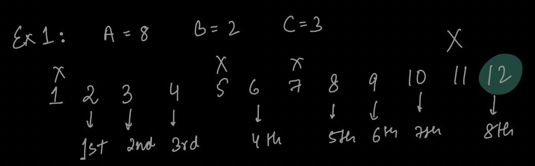
A = 8
B = 2
C = 3

A * B = 16
A * C = 24
So, our answer will be within range [1 to 16]

Que: How many multiples of B, C will be within range [1 to x]? => x/B + x/C - x/LCM(B,C)$

The LCM of 'b' and 'c' represents the smallest common multiple of 'b' and 'c' such that any number that is divisible by both 'b' and 'c' will be a multiple of their LCM and we will have to subtract it

Example:

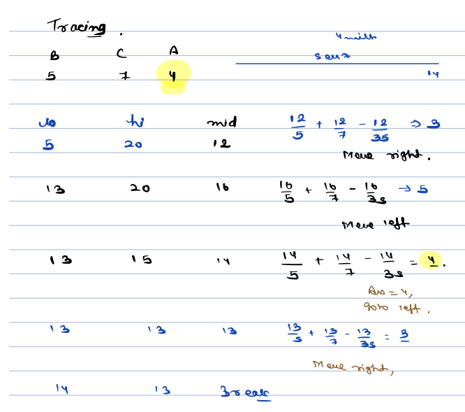
A = 5
B = 3
C = 4
Range => [1 to 15]

Multiples

=> 15/3 + 15/4 - 15/LCM(3,4)

=> 5 + 3 + 1 = 7 [3, 4, 6, 8, 9, 12, 15]

Que: How to calculate LCM(B,C) ?

LCM(B,C) = (B * C) / GCD(B,C) [We know how to calculate GCD!]

Can we apply Binary Search ?¶

Search Space => [1 to A * min(B,C)]

Target => Ath Magical Number

Condition =>

Say we land at mid.
To check mid is magical, we need to know how many magical numbers are there in the range [1, mid].
Compare with A: If the count is more than A, it means we need to search in the lower range [low, mid-1].
Otherwise, if count is < A, we need to search in higher range
If count == A, then we store mid as answer, and go left.

Pseudocode:¶

int count(x, B, C) {
    return x/B + x/C - x/LCM(B,C);
}

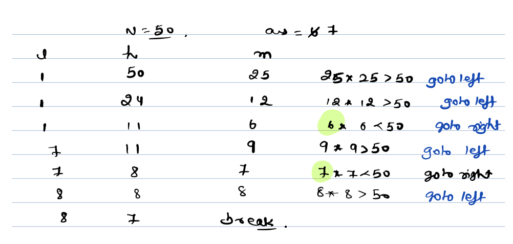
int magical(A, B, C) {
    l = 1, h = A * min(B,C)
    while(l <= h) {
        m = l + (h-l)/2;
        if(count(m,B,C) > A) {
            h = m-1;
        }
        else if(count(m,B,C) < A) {
            l = m+1;
        }
        else {
            ans = m;
            h = m-1;
        }
    }
    return ans;
}

Question¶

What is the time complexity of the binary search approach for finding the a-th magical number in terms of A, B, and C?

Choices

O(A)
O(log A)
O(A * B * C)
O(log(A * B * C))

Problem 4 Finding median of array¶

What is Median?

The median of an array is the middle element of the array when it is sorted. For arrays with an odd number of elements, the median is the value at the exact center. For arrays with an even number of elements, the median is typically defined as the average of the two middle elements. It's a measure of central tendency and divides the data into two equal halves when sorted.

Brute-Force Algorithm to Find the Median of an Array:¶

Sort the given array in ascending order. You can use any sorting algorithm (e.g., bubble sort, insertion sort, quicksort, or mergesort).
Calculate the length of the sorted array, denoted as n.
If n is odd, return the middle element of the sorted array as the median (e.g., sorted_array[n // 2]).
If n is even, calculate the average of the two middle elements and return it as the median (e.g., (sorted_array[n // 2 - 1] + sorted_array[n // 2]) / 2).

def find_median_brute_force(arr):
    # Step 1: Sort the array
    sorted_array = sorted(arr)

    # Step 2: Calculate the length of the sorted array
    n = len(sorted_array)

    # Step 3: Find the median
    if n % 2 == 1:
        median = sorted_array[n // 2]
    else:
        median = (sorted_array[n // 2 - 1] + sorted_array[n // 2]) / 2.0

    return median

Warning

Please take some time to think about the Binary Search approach on your own before reading further.....

Binary Search Approach:¶

The Binary Search technique can be harnessed to find the median of two sorted arrays by partitioning the arrays in such a way that the elements on the left side are less than or equal to the elements on the right side. The median will be either the middle element in a combined array (for an odd number of total elements) or the average of two middle elements (for an even number of elements).

Example: Finding Median of Two Sorted Arrays¶

Scenario:

Consider the two sorted arrays: nums1 = [1, 3, 5] and nums2 = [2, 4, 6]. We want to find the median of the combined array.

Intuition:

Combined Sorted Array: To find the median of two sorted arrays, you can think of combining them into a single sorted array. The median of this combined array will be our solution.
Partitioning: The key idea is to partition both arrays into two parts such that:
The elements on the left side are smaller than or equal to the elements on the right side.
The partitioning should be done in such a way that we can calculate the median easily.

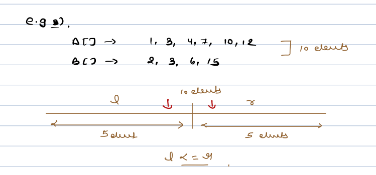
Binary Search: To achieve this, we can perform a binary search on the smaller array (in this case, nums1). We calculate a partition point in nums1, and then we can calculate the corresponding partition point in nums2.

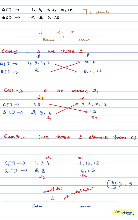
Median Calculation: Once we have the partitions, we can calculate the maximum element on the left side (max_left) and the minimum element on the right side (min_right) in both arrays. The median will be the average of max_left and min_right.

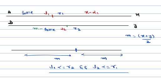
Handling Even and Odd Lengths: Depending on whether the total length of the combined array is even or odd, the median calculation varies. If it's even, we average the two values; if it's odd, we take the middle value.

Solution:

We start by calculating the total length of the combined arrays to determine if the median will be even or odd.
Then, we use binary search on the smaller array (nums1) to find a partition point that satisfies the conditions mentioned earlier. This ensures that elements on the left are smaller or equal to elements on the right.
We calculate max_left and min_right for both arrays based on the partitions.
Finally, we calculate the median as the average of max_left and min_right.

Binary Search:

Initialize left = 0 and right = len(nums1) = 3.
Iteration 1:
Calculate partition_nums1 = $(0 + 3) / 2 = 1$.
Calculate partition_nums2 = $(6 + 1) / 2 - 1 = 2$.
Calculate max_left_nums1 = 1 and max_left_nums2 = 2.
Calculate min_right_nums1 = 3 and min_right_nums2 = 4.
Since 1 <= 4 and 2 <= 3, we have found the correct partition.
Since the total length is even (6), the median is the average of the maximum of left elements and the minimum of right elements, which is $(2 + 3) / 2 = 2.5$.

Pseudocode:¶

Here's a simplified pseudocode representation of finding the median of two sorted arrays using Binary Search:

function findMedianSortedArrays(nums1, nums2):
    if len(nums1) > len(nums2):
        nums1, nums2 = nums2, nums1

    total_length = len(nums1) + len(nums2)
    left = 0
    right = len(nums1)

    while left <= right:
        partition_nums1 = (left + right) / 2
        partition_nums2 = (total_length + 1) / 2 - partition_nums1

        max_left_nums1 = float('-inf') if partition_nums1 == 0 else nums1[partition_nums1 - 1]
        max_left_nums2 = float('-inf') if partition_nums2 == 0 else nums2[partition_nums2 - 1]

        min_right_nums1 = float('inf') if partition_nums1 == len(nums1) else nums1[partition_nums1]
        min_right_nums2 = float('inf') if partition_nums2 == len(nums2) else nums2[partition_nums2]

        if max_left_nums1 <= min_right_nums2 and max_left_nums2 <= min_right_nums1:
            if total_length % 2 == 0:
                return (max(max_left_nums1, max_left_nums2) + min(min_right_nums1, min_right_nums2)) / 2
            else:
                return max(max_left_nums1, max_left_nums2)
        elif max_left_nums1 > min_right_nums2:
            right = partition_nums1 - 1
        else:
            left = partition_nums1 + 1

Analysis:¶

In each iteration, the algorithm adjusts the partition positions based on the comparison of maximum elements on the left side with minimum elements on the right side of the partitions. The Binary Search nature of this algorithm leads to a time complexity of O(log(min(m, n))), where m and n are the lengths of the two input arrays.

Use Cases:¶

The concept of finding the median of two sorted arrays is crucial in various fields, including data analysis, algorithms, and statistics.

Observations¶

Sorted Arrays: Binary Search excels in sorted arrays, capitalizing on their inherent order to quickly locate elements.
Search Space: Identify the range within which the solution exists, which guides setting up the initial search range.
Midpoint Element: The middle element provides insights into the properties of elements in different subranges, aiding decisions in adjusting the search range.
Stopping Condition: Define conditions under which the search should stop, whether an element is found or the search range becomes empty.
Divide and Conquer: Binary Search employs a "divide and conquer" strategy, progressively reducing the problem size.
Boundary Handling: Pay special attention to handling boundary conditions, avoiding index out-of-bounds errors.
Precision & Approximations: Binary Search can yield approximate solutions by adjusting the search criteria.